A simple example: the lactose operon

Description of the biological problem

The lactose operon is one of the most studied example in the regulation of proteins production. In Escherichia coli, the operon [1] encodes three different genes named lacZ, lacY and lacA from which the two firsts are the most importants. LacZ codes for a protein that hydrolizes lactose to produce glucose and galactose, which are themselves used by the cell as carbon sources. LacY encodes a permease, a protein which pumps the lactose into the cell. Both of these proteins need to be synthesized by the cell to use the lactose as an energy source, but as this is costly, and less efficient than using the glucose directly, the cell manages to produce them only in presence of lactose and in absence of glucose.

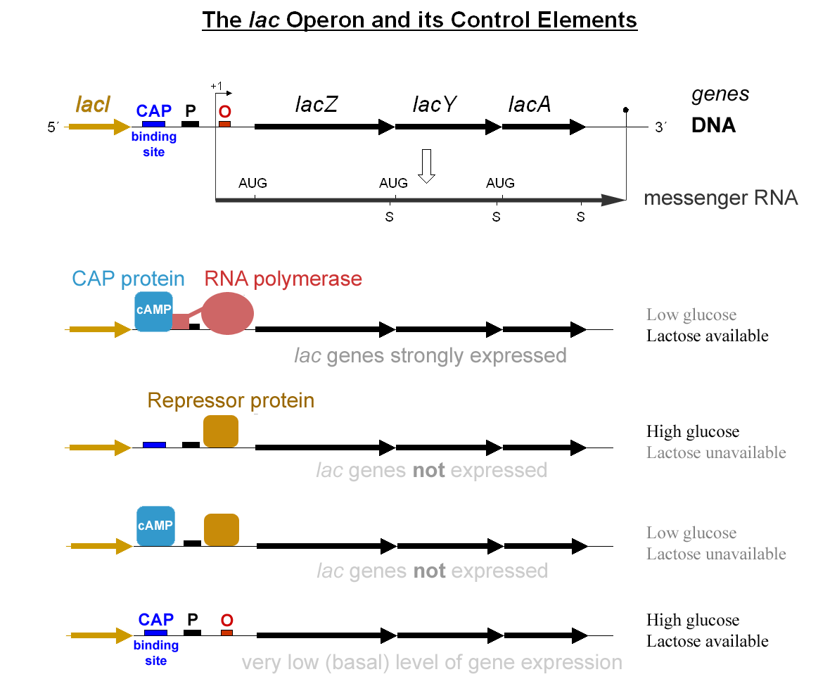
Figure 1: Scheme presenting the main elements of the lactose operon along the DNA strain (top), and the state of the operon through several external conditions (bottom). Published on Wikimedia by G3pro and Tereseik.

Cells have thus designed a logical gate, schematically shown in Figure 1 , to compute the binary function: lactose and no glucose that controls the expression of the whole operon. The biological strategy is the following: near the operon, the gene lacI encodes a repressor of the operon which is constitutively expressed so that by default, the operon is turned off. When lactose is present in the medium, a closed form, the allolactose is also present and will bind to the lacI repressor, thus impeding it to block the operon. It is now possible to expressed the operon but there is still no activation. The activator, the CAP protein, is indeed in an active form only in the presence of cAMP which is produced in absence of glucose [2]. As long as glucose is present, the operon is still silent and it is only when glucose become rare that cAMP goes high, thus activating the CAP protein which activate the operon and thus the production of the needed proteins.

Hereafter, we will run our genetic algorithm to optimize a function close from the logical gate corresponding to the lac operon, that is: \(x,y \mapsto x~\&~\neg~y\) (\(x~\text{nand}~y\)), the link with the biology of the real lac operon would nonetheless ask more work than will be presented here.

Implementation in the algorithm

Remark

All files, functions and variables names along with terminal commands will be printed using the LaTeX environment verbatim and display with this particular font.

Two mains questions need to be answered in order to configure the algorithm for a particular problem. What? and How? : What is the precise function we need to optimize in order to describe the problem? and How the solution is allowed to be found by the algorithm? The first will be mainly described by the C code files like init_history.c and fitness.c while the second will be solved through the tuning of the various parameters in the so called init*.py file.

The init_history.c file describes the form of the input(s) that will be feed into the network. This is done through the construction of the double array isignal[time][n_cell][n_input] which indicates the concentration of the various input with respect to the time and cell.

In our case, we have two inputs that will represent the concentration of glucose and lactose and will be taken as binary functions (each sugar has a concentration of \(0.0\) or \(1.0\)) which follow a random sequence of presence and absence, the time being spent in each state uniformly drawn between \(10\) and \(60\) seconds (see figure [fig:response_lo]).

The fitness.c file intend to process the output of the integrator which is rounded up in the double array named history indexed in the following way: history[Species][Time][Cell]. The variables trackin and trackout keeps in memory the label of the inputs and outputs species. The fitness is directly printed out by the treatment_fitness function. (Note however, that treatment_fitness is a void, fitness is passed with the printf("%f",fitness); statement.)

For lac operon simulation, each try of the integrator is treated independantly and follow the time course of the input and output to determine the times at which production is needed (that is when there is lactose and no glucose) and the concentration of the output at that time. We then have chosen to compute the mutual information [3] between \(\text{lactose}~\&~\neg \text{glucose}\) and the concentration of the output.

Finally, the init*.py file indicate the mutation rates of the different interactions, the number of networks in the population, the number of generation of the simulation, the initial network from which we want to start and so on.

In the case of the lac_operon, we will ask the algorithm to use only protein-protein interaction (PPI) and repression/activation of gene (TFHill) and put to zero the parameters indicating the appearance of other interactions, for example:

random_Interaction('Degradation') = 0
random_Interaction('Phosphorylation') = 0

which control the rate at which new degradations and phosphorylations are added to the network to be probed by the evolution.

---

Each of this file has to be put in a single folder (in our case lac_operon/) in order to be found by the algorithm. Evolutionary procedure is now simply launched by running the

python run_evolution.py -m lac_operon

command line while in the main folder. The algorithm will now display a lot of more or less important stuff in your terminal. The most interesting are the generation number which indicate at which point of your simulation you are. When accustomed to it, the Best_fitness is an interesting variable to look at to know if the condition you defined actually allow the algorithm to find valid solution for the problem. Finally, every line starting by ERROR needs of course your special attention.

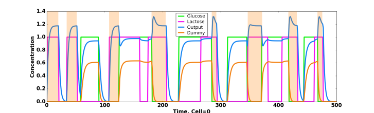
Figure 2: Detailed response of the network presented in Figure 3 A, colors correspond between the two figures. Orange shades indicate the time at which response is waited.

A word about fitness

In order for the evolutionary procedure to give meaningful results, a special attention need to be given to design a proper fitness function. There is several reasons for this particular importance but the main one is that the algorithm will only try to solve the exact problem you have defined – i.e. minimize the fitness function you have provided – which is usually different from the actual task you have in mind.

For example, one of the solution proposed by the algorithm for the lac_operon fitness proposed earlier (the mutual information between the output concentration and the \(\text{lactose}~\&~\neg \text{glucose}\) function) was to use lactose as a weak activator of the output and glucose as… a strong activator of the output! When looking at the time course of the output concentration, it makes plain sense because the concentration is near zero when there is no sugar, goes to one when there is only lactose and saturate around two when there is either glucose only or when both sugare are presents. Thus if the concentration is around one you know that you have lactose and no glucose. You can extract the whole information about the \(\text{lactose}~\&~\neg \text{glucose}\) function from the output concentration which is the task we ask for, even if the answer was quite surprising.

This also mean that you will often want to modify your fitness function after a first bunch of runs to be more explicit or to try a different fitness function. To avoid being rapidly lost between your different simulation, you can look at the Seed*/log_fitness.c file for a reminder of the fitness used at this time.

A second remark about fitness is that the function should goes smoothly from the low fitness landscape to the region you want to explore, that is the fitness function should already rewards the first steps toward the solution. Otherwise, the algorithm will be stuck in the low level region and cannot even start to optimize. This question covers a broad range of litterature both in evolutionary biology and genetic algorithm computer science around the fitness-landscape shape question with suggestive names such as mount Fuji, house of cards or golf-course. It is usually not a big deal but could bring you some surprise if you don’t keep it in mind.

How to read and interpret results

Now that your computer has run several simulations it is time to analyse them to decipher the output of the evolutionary algorithm. The first thing to look at is the time course of the fitness for several runs, to show the fitness of the first run, you can either use the Analyse Run notebook or use the Simulation class.

Make sure to check several runs to know the typical fitness of a successful or failed run, this will discard the cases where the evolutionary algorithm has been stuck and doesn’t have enough time to converge.

To study a particular network, you can now type network(500) if you want to display the state of the best network in the population at generation \(500\) (the end of the simulation given our init*.py files). It may be small and concise but usually it’s not, evolutionary procedure tends to accumulate a lot of uninteresting interactions and species – the famous DNA junk? –that may be ignored. Anyway, this is the raw result of the evolution. It will print out the file directory where the network has been saved for later analysis.

You can from there read and write network (with the read and write function), compute the fitness (with the fitness function) and even look at the time course of the species for a particular realisation of the fitness computation. If net is your network, just type fitness(net, plot=True). You can also plot a network using net.draw().

Finally, you can also add homebrew function to analyse your evolutionary result by adding a analyse.py file in the project folder. It will be imported with analyse_network through the name spec.

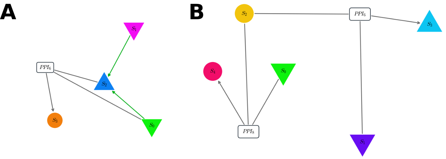
Figure 3: Pannels A. and B. shows two typical topologies of the final result of the algorithm trying to optimize our mutual-information fitness. In both pannel, inputs are species \(0\) (glucose) and \(1\) (lactose) (down-triangle) and output is the up-triangle. A. Both sugars regulate positively the output, but the glucose also form a dimer with it thus impeding the response. The time course of this network is displayed in Figure 2. B. Here a single species (S2) can form two complexes, one very strongly with the glucose (S4), and another weaker with the lactose (S3). The former complex being the output.

In our case, out of 10 runs, 80% ended on 2 main different topologies (after pruning) both performing correctly, that is the fitness plateau around \(-0.8\) on a scale of \(0\) to \(-1\). Four correspond to the network of Figure 3 -A while four other looks like the one in Figure 3 - B. I let up to you the biological interpretation of these results [4] but the first obvious feature is the uniformity of the solution. Nearly all the successfull runs show very similar patern indicating that the biological grammar available actually imposes strong constraints on the possibles solution to a particular problem.

Geometry

New interactions

[1]	In genetics, an operon is a functioning unit of DNA, it designates a cluster of genes under the control of a single promoter.

[2]	For curious reader, the reason why, when energy tends to rarify, the cell suddenly produces an extraodinary amount of seemingly useless proteins is still an active question!

[3]	The mutual information of two random variables is a way to quantify the information I can extract about one variable by measuring the second.

[4]	Just a hint, for case B it seems to me that species 2 should be considered as the DNA strain!

[5]	As a particular example, suppose you want to buy a chair. You want it comfy, robust and cheap, if you can have more comfort without decreasing robustness nor increasin price… that’s better, but between the cheap one and the costly but better, it is ultimately a matter of taste.